個人資訊

吳俊逸
訪客 (634482), 推薦 (3)
文章 (377)
回應 (1)
文章分類
Trademark (11)
Industry 4.0 (32)
NLP (10)
AI (46)
Patent (110)
Course (20)
Supply chain (44)
uncategorized (38)
最新文章
Python Model Evaluation
by 吳俊逸 2018-05-29 14:47:44, 回應(0), 人氣(2565)
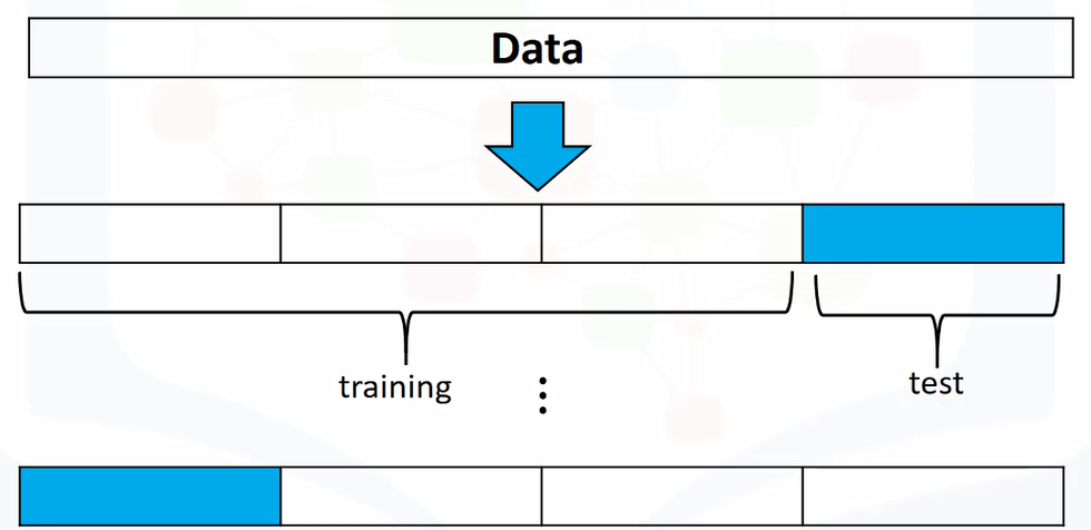
Training and Testing
y_data=df['price']
x_data=df.drop('price',axis=1) #drop price data in x data

from sklearn.model_selection import train_test_split
x_train, x_test, y_train, y_test = train_test_split(x_data, y_data, test_size=0.15, random_state=1)
print("number of test samples :", x_test.shape[0])
print("number of training samples:",x_train.shape[0])
Let's import LinearRegression from the module linear_model
from sklearn.linear_model import LinearRegression
lre=LinearRegression()
lre.fit(x_train[['horsepower']],y_train)
lre.score(x_train[['horsepower']],y_train) >> 0.6377940995166673
lre.score(x_test[['horsepower']],y_test) >> 0.707688374146705
from sklearn.model_selection import cross_val_score
Rcross=cross_val_score(lre,x_data[['horsepower']], y_data,cv=4)
print("The mean of the folds are", Rcross.mean(),"and the standard deviation is" ,Rcross.std())
The mean of the folds are 0.522009915042119 and the standard deviation is 0.2911839444756029
lr=LinearRegression()
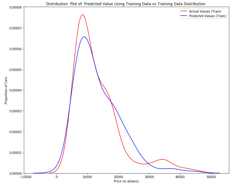
lr.fit(x_train[['horsepower', 'curb-weight', 'engine-size', 'highway-mpg']],y_train)
yhat_train=lr.predict(x_train[['horsepower', 'curb-weight', 'engine-size', 'highway-mpg']])
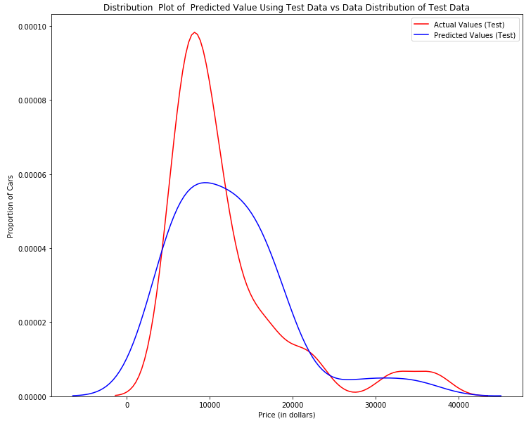
yhat_test=lr.predict(x_test[['horsepower', 'curb-weight', 'engine-size', 'highway-mpg']])
import matplotlib.pyplot as plt
import seaborn as sns
DistributionPlot(y_train,yhat_train,"Actual Values (Train)","Predicted Values (Train)",'Title')
DistributionPlot(y_test,yhat_test,"Actual Values (Test)","Predicted Values (Test)",Title)
from sklearn.preprocessing import PolynomialFeatures
x_train, x_test, y_train, y_test = train_test_split(x_data, y_data, test_size=0.45, random_state=0)
pr=PolynomialFeatures(degree=5)
x_train_pr=pr.fit_transform(x_train[['horsepower']])
x_test_pr=pr.fit_transform(x_test[['horsepower']])
poly=LinearRegression()
poly.fit(x_train_pr,y_train)
yhat=poly.predict(x_test_pr )
PollyPlot(x_train[['horsepower']],x_test[['horsepower']],y_train,y_test,poly,pr)
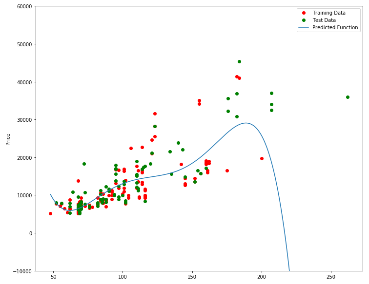
poly.score(x_train_pr, y_train) >> 0.5567716899817778
poly.score(x_test_pr, y_test) >> -29.871838229908324 << Overfitting
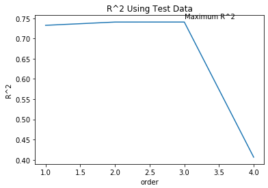
Let's see how the R^2 changes on the test data for different order polynomials and plot the results:
Rsqu_test=[]
order=[1,2,3,4]
for n in order:
pr=PolynomialFeatures(degree=n)
x_train_pr=pr.fit_transform(x_train[['horsepower']])
x_test_pr=pr.fit_transform(x_test[['horsepower']])
lr.fit(x_train_pr,y_train)
Rsqu_test.append(lr.score(x_test_pr,y_test))
plt.plot(order,Rsqu_test)
plt.xlabel('order')
plt.ylabel('R^2')
plt.title('R^2 Using Test Data')
plt.text(3, 0.75, 'Maximum R^2 ')
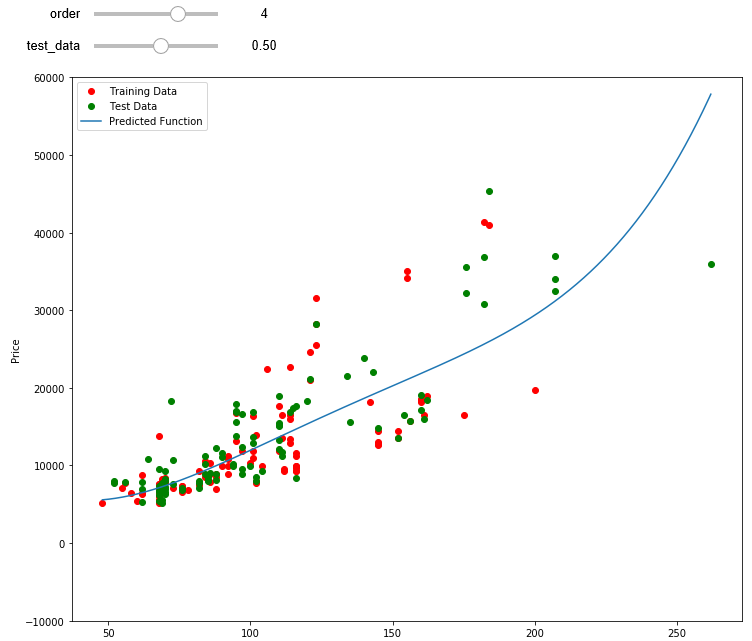
def f(order,test_data):
pr=PolynomialFeatures(degree=order)
x_train, x_test, y_train, y_test = train_test_split(x_data, y_data, test_size=test_data, random_state=0)
x_train_pr=pr.fit_transform(x_train[['horsepower']])
x_test_pr=pr.fit_transform(x_test[['horsepower']])
poly=LinearRegression()
poly.fit(x_train_pr,y_train)
PollyPlot(x_train[['horsepower']],x_test[['horsepower']],y_train,y_test,poly,pr)
interact(f, order=(0,6,1),test_data=(0.05,0.95,0.05))
from sklearn.linear_model import Ridge
RigeModel=Ridge(alpha=0.01)
RigeModel.fit(x_train_pr,y_train)
yhat=RigeModel.predict(x_test_pr)
from sklearn.model_selection import GridSearchCV
parameters1= [{'alpha': [0.001,0.1,1, 10, 100, 1000,10000,100000,100000]}]
RR=Ridge()
Grid1 = GridSearchCV(RR, parameters1,cv=4)
Grid1.fit(x_data[['horsepower', 'curb-weight', 'engine-size', 'highway-mpg']],y_data)
BestRR=Grid1.best_estimator_
BestRR.score(x_test[['horsepower', 'curb-weight', 'engine-size', 'highway-mpg']],y_test)
Example:
parameters2= [{'alpha': [0.001,0.1,1, 10, 100, 1000,10000,100000,100000],'normalize':[True,False]} ]
Grid2 = GridSearchCV(Ridge(), parameters2,cv=4)
Grid2.fit(x_data[['horsepower', 'curb-weight', 'engine-size', 'highway-mpg']],y_data)
BestRR2=Grid2.best_estimator_
BestRR2.score(x_test[['horsepower', 'curb-weight', 'engine-size', 'highway-mpg']],y_test)
附件: